Net Change SDEVs
"Net Change SDEVs" uses standard deviations of percent net change over a sample period of time. This allows the trader to see historically, to an exact probability, where price has closed for that duration of timeframe. This allows the trader to anticipate key reversal points for any given timeframe.
The below metrics were calculated from a 20yr sample, 2004-2024. Times listed are in Eastern Standard.
This is the bread and butter of my edge. To understand what these are, we need to go over statistics/probabilities really quick. Don't worry though, I will make it easy to understand.
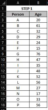
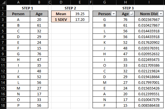
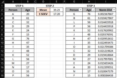
Most things can be broken down to distribution probabilities. Example, a group of 16 people at different ages. We can find where ~70% of the people reside by age. Say the ages range between 15yrs and 76yrs.
Step 1
We need to collect the sample.
What are net change standard deviations?

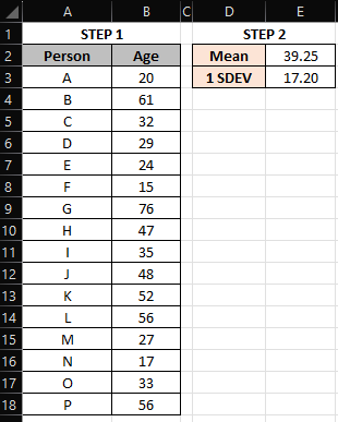
Step 2
Next we need to get the +/- 1 SDEV by simply using the “STDEV.P” function. This is all you need to now understand the variance in the data set. You can break this down to 0.5 increments using basic math.
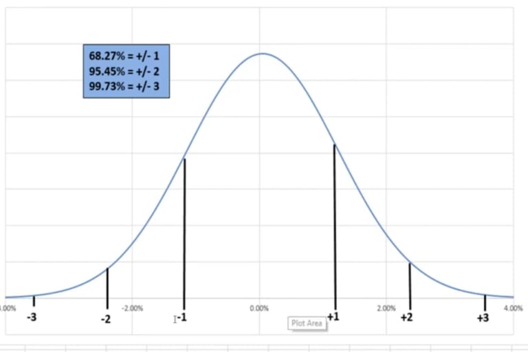
While not required to make a trading related indicator, you can further break down the data to create a visualization via creating a bell curve. We need to get the mean (average). This will be using the “AVERAGE” function in MS Excel. The 1 standard deviation will represent the variance from the mean to a +/- 1 standard deviation, which equates to 68.2689% or roughly 70%. This will be shown later. What this standard deviation is showing is there is a mean of 39.25 years old and 70% of the sample resides within +/- 17.20 yrs from the mean. So 70% of people fall within 22yrs old to 56yrs old.

Step 3
Finally, we need to get the normal distribution of each person relative to where they fall in the sample. This will be using the “Norm.Dist” function in excel. The formula is as follows:
=Norm.Dist(x, mean, standard_dev, cumulative)
x = persons age
mean = sample mean calculated earlier
standard_dev = 1 SDEV calculated earlier
cumulative = false
Completed for Person A, it looks like this:
=NORM.DIST(C30,$C$24,$C$25,FALSE)
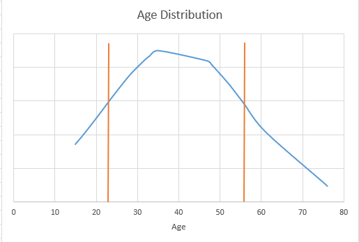
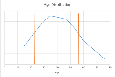
Finally, we will create the bell curve chart using the Age and Norm Dist columns, and using a “Scatter with smooth lines” chart. The final product is shown below. The orange vertical lines represent the +/- 1 SDEV, where ~70% of the people reside.
How do I apply this to the market?
So far I showed you the basics of taking a sample of data and creating a z-score (1 SDEV). I also showed you how to create a bell curve for the sample. But how does one apply this to a chart of an asset? I look at distribution metrics for % net changes of specific timeframes. This logic can be applied to any timeframe, but I only apply it to monthly, weekly, daily and 1-hour timeframes. In the example below I will be discussing the daily timeframe.
If we get the daily % net change for the Nasdaq-100 e-mini over the last 20 years, we have a sample of daily net changes, roughly 5,000 data points to work with, creating a much smoother bell curve as shown below. We can than calculate the +/- 1 SDEV. This will give us a +/- % net change from the daily session open. For the last 20 years, the 1 SDEV is +/- 1.376%. Meaning ~70% of the time the session closes within the zone of +/- 1.376% net change. Using this we can also calculate +/- deviations to other degrees like the 0.5, 1.5, 2.0, etc. just using simple multiplication and division. If you want the 2.0 deviation, than just multiple 1.376% x 2.
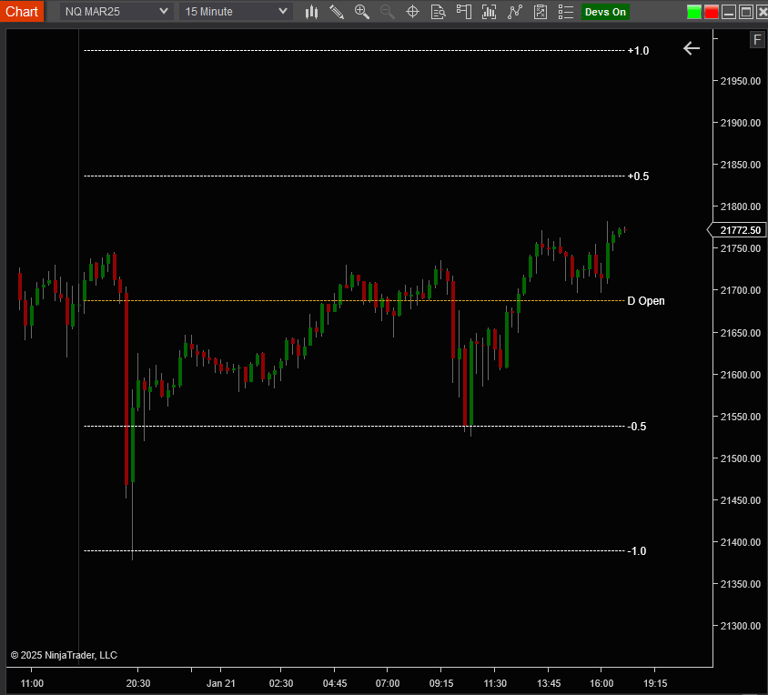
As the daily session opened this particular day, price trended down and reverted off the -1.0 deviation. From a probability perspective, there is a 68.27% probability that the session will close between +1.0 and -1.0. There is also a 84.13% probability that the session will close specifically above -1.0. These percentages are calculated via my indicator, but you can also use a web based z-score to percentile calculator. Every z-score (SDEV Value) has a specific percentage of probability, I personally just use increments of 0.5. Additionally, I use a custom field that returns the exact z-score price is currently at and its associated probability.
Price traded back up to the mean (session open), than proceeded to trade down again and pivoted off the -0.5 deviation. From a probability perspective, there is a 38.30% probability that the session closes between +0.5 and -0.5. There is also a 69.15% probability that the session will close above -0.5 specifically.
These pivot points are quantitative. They are math derived. If you pay attention to them, you will see the pivotal nature they present. This is likely due to other larger money movers utilizing something similar in their quantitative approach. This logic can be applied to any timeframe. It will provide expectations of price both from a reversion perspective and a target move perspective. For example, it is unlikely that price goes to the +/- 1.5 daily distribution deviation in any single given day, just due to the fact that the probability of the reversion is so high well before that, thus any bias you have should take this into account. A move beyond a +/- 1 SDEV move, would be considered outlier, and a early indication of a trend day.
If you have any questions about this, please feel free to ask.
I created a custom indicator in NinjaTrader that does all this for me, for the various timeframe I want to see. This indicator is not public and I will not share it, but everything I have talked about on this page is how its derived. When we apply this concept to a chart, essentially rotating the bell curve 90 degrees to its side, it looks like such.
I refer to this as "rubber band theory". The farther price stretches from the mean (timeframe open), the more reversion tension is placed on price relative to its historical performance. There will be times where the rubber band snaps (outlier days) and price trends in a single direction. These trend days are often spotted early when price does not pivot or consolidate at the +1.0, but instead extends past it like it doesn't exist. Price spends more time ranging than expanding, thus you will see more pivots at these levels than expansion through.